FAST: A High-Throughput Spectrograph for the Tillinghast Telescope

1.0 Introduction

1.1 Spectrograph Characteristics
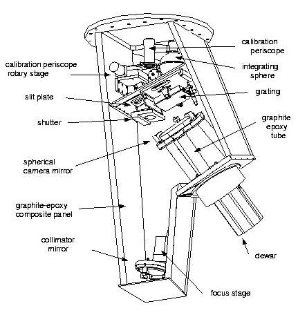
FAST has a conventional plane reflection grating geometry with an off-axis parabolic collimator and a Schmidt camera. The focal length of the collimator is 963 mm and the effective focal length of the camera is 328 mm, giving a reduction of 2.93, corresponding to a scale of 0.57 arcsec/15 pixel along the slit. The unvignetted slit length is 3 arcminutes, or 13.72 mm at the slit. The angle between the collimated beams arriving at and leaving the grating is 35. The layout of the spectrograph is:

1.2 Gratings
FAST is designed to accept gratings with rulings between 300 and 1200 lines per mm in first order. Table 1 gives the resolutions and spectral coverages for various gratings with a 53 mm long CCD, such as the current one (see Sect. 1.4). The spectrograph will vignette at the spectral extremes if a grating with an anamorphic factor exceeding 1.3 is used. This corresponds to a 1200 line grating centered at H, so a 1200 line grating in the extreme red entails a modest loss in efficiency.

Ruling	2 Pixel Res	Spectral Coverage	2 Pixel Slit Width
300 gpm	2.94	4000	1.21 arcsec
600 gpm	1.48	2000	1.25 arcsec
1200 gpm	0.75	1000	1.52 arcsec

We have 3 gratings available: a 300 and 600 line grating blazed at 4750 , and a 1200 line grating blazed at 5700 . The 300 and 600 line gratings have 50% efficiency limits of 3500 and 8000 , and the 1200 line grating has 50% efficiency limits of 4000 and 10000 . The gratings can be changed manually through the access hatch of the spectrograph.

1.3 Efficiency
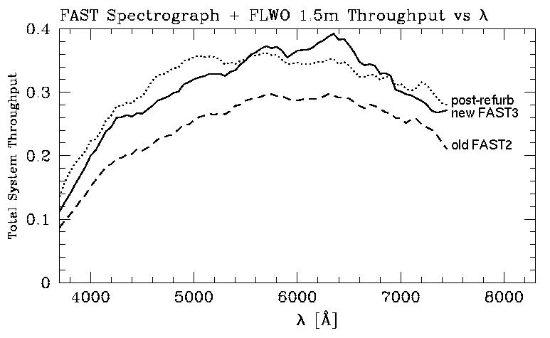
FAST was designed for high throughput between 3700 and 9000,making use of high efficiency antireflection coatings and UV enhanced, over coated silver coatings for the mirrors. With the thinned, back-side illuminated CCD with antireflection coating (see next section), the peak efficiency (including detector) reaches ∼ 40%. The figure below shows the efficiency versus wavelength with CCD FAST3, compared to its predecessor FAST2. (Measurements by Perry Berlind 07/24/06, analysis by Warren Brown 07/25/06.)

1.4 CCD Characteristics
Since June 2006, the CCD is FAST3, a backside-illuminated chip with a blue-enhanced AR coating, 2688x512 UA STA520A chip with 15μ pixels. John Geary and Steve Amato mounted and tested the new CCD. The CCD operating temperature is ∼ -110 C, giving a dark current of less than 1 electron/hr/pixel. The readout noise of the CCD is ∼ 4.4 electrons RMS. The CCD gain for FAST3 is currently set to 0.8 electrons per ADU. The readout time is ∼ 25 sec for the full, unbinned chip.

1.5 Slits
There are 5 fixed-width slits available: 1.1, 1.5, 2, 3, and 5 arcseconds wide. These can be changed manually through the access hatch of the spectrograph. The resolution versus slit width for a 300 gpm grating is given in the following table. It will be slightly better with more finely ruled gratings.

Slit Width	Pixels
(arcsec)	FWHM
1.1	2.0
1.5	2.3
2.0	2.8
3.0	4.2
5.0	7.4

1.6 Blocking Filters
We have two long pass filters available with cutoffs of 3700 and 5000 . These are mounted in a slide between the slit and the shutter.

1.7 Automated Features
The collimator focus and the comparison stage can be remotely operated via computer, as can the calibration lamps (He-Ne-Ar and Incand).

2.0 Calibration Lamps
The wavelength comparison lines are produced by a He-Ne-Ar lamp (which lost most of its He and looks like Fe-Ne-Ar).
The following figure shows a typical He-Ne-Ar spectrum taken with the 300 gpm grating:

3500-7500 jpeg / postscript

The following 5 Figures are a detailed spectral line atlas covering most of the useful spectral range with the 300 gpm grating:

3600-4700 jpeg / postscript --- 4500-5500 jpeg / postscript
5300-6300 jpeg / postscript --- 6100-7100 jpeg / postscript
6900-7900 jpeg / postscript

and another 4 with the 1200 gpm grating to resolve some blended lines:

3400-4500 jpeg / postscript --- 4300-5400 jpeg / postscript
5200-6300 jpeg / postscript --- 6100-7200 jpeg / postscript

The incandescent lamp unfortunately is weak below 4500 , even after the introduction of a color balancing filter. Bluer filters are available, but the filters we tried introduced strong variations in intensity with periods of several hundred . We felt that most users would prefer to make multiple flat exposures rather than deal with strong short period intensity variations. The incandescent lamp is quite bright, requiring an exposure of 16 seconds (in bin x1).

All lamps are fed into an integrating sphere to scramble the lamp outputs and then pass through an achromatic lens to simulate the exit pupil of the telescope. This should produce an accurate calibration. Please be aware, however, that no calibration lamp is perfect, and that wavelength shifts between the sky and the lamps will be present at some level. A good way to check for offsets is to look at the calibrated wavelengths of known strong lines in the spectrum of the night sky. We have verified that the spectrograph flexure as measured by the comparison lamps tracks the flexure measured by night sky lines quite accurately.

All light from the integrating sphere passes through a 1 mm thick BG-14 filter. This reduces the intensity of the strong red comparison lines and provides some color balancing for the incandescent lamp.

3.0 Focusing and Wavelength Stability
The spectrograph case is constructed from low-expansion graphite-epoxy composite panels with a coefficient of thermal expansion less than 25% that of aluminum. During the first run of FAST on the telescope we noticed only a small defocus resulting from a change from the lab temperature of 20 to the 0C typically encountered at night. As a result, the spectrograph will stay in focus over the temperature changes occurring on a typical run. The graphite epoxy composite will expand and contract with humidity changes, but this is a slow process that should not be noticeable in a single run.

Each step of the stepper motor that controls the collimator focus corresponds to a movement of 10 . Given that the telescope is f/10, that the reduction is 2.9 and the 15-μ pixel size, it will probably not be necessary to focus in moves smaller than 10-20 steps.

FAST was designed to achieve good short term stability, that is: good stability over the course of the longest anticipated exposure, about one hour. There are two major contributors to this stability: mechanical flexure and thermal shifts. The measured mechanical flexure averages 0.3 pixel per 15μm), which corresponds to an hour of tracking an object. For short exposures, it will probably be necessary to take only a single HeNeAr comparison exposure. The flexure is largest moving from E to the zenith and N to the zenith, and almost absent moving to the S from the zenith. There is a small amount of hysteresis (∼0.2 pixels) as the telescope returns to the zenith from different directions.

We have measured the thermal stability of the spectrograph in the laboratory and find a 0.2 pixel/C shift, close to what we calculated should be present. Given that the night-time temperature changes are typically 0.25C/hour during the night, this should not be significant even for a long exposure. The thermal time constant of the spectrograph is about 3.5 hours, so if the dome is allowed to heat up significantly during the day, it would be wise to open the dome as soon as possible if the maximum stability is required. Opening the dome near sunset will also help the seeing.

4.0 Changing Slits and Gratings
Changing gratings requires great care. In general, you should ask the staff to change the gratings for you during the day. In special cases, you may obtain permission to change slits or gratings after receiving training from the day staff and from the remote observers. Also, do read and make sure you understand the instructions below as a first step. If you are feeling clumsy or groggy, do not ever attempt to change gratings. Gratings cost $5000 or more and their replacement time is long.

Gratings and slits are installed through the single removable panel on the spectrograph. This panel is secured with two handles that rotate by 90 between open and closed. The access panel must be completely removed and placed in a safe location before proceeding further. The slits are held in place by spring-loaded plungers; the slit is simply pulled out by grasping its handle. The new slit should be inserted reflective side up and pushed home. The filter slide, mounted below the slit, is removed and installed in the same fashion.

Before removing a grating, remove heavy jackets as the access port will not accommodate down jackets and heavy sweaters. Remember that vulnerable optics are exposed beneath the grating. Please do not drop your flashlight, pens, etc. into the spectrograph!

Gratings are stored inside the chamber. You will find them with their covers closed. These are held closed by magnets. They can be pried open with gentle force, once the grating is mounted on the spectrograph. The first step of removal of a grating must be to close its cover. To close it, just swing the cover up until the magnets catch.

The grating is secured with two bolts, one in back and one just inside the access panel. These two bolts must be loosened so that the grating rests on the slides that guide it into position. The arm that carries the forward bolt is then pushed up and rotated 90 to the right until the spring plunger seats, holding it out of the way. The grating can then be carefully removed and stowed away. Make sure you look inside the spectrograph with adequate light to ensure the grating cover is closed, otherwise you may add your own fingerprints to the collection already on some of the gratings. Note that if you ever do this, you should not attempt to clean the grating in any way, and you should notify the staff of the mishap.

To install the new grating, reverse the removal procedure. Take care that the grating does not twist from side to side as it is inserted or it will bind. Tighten the two grating bolts gradually, alternating so that the grating seats properly in its kinematic mount. Do not overtighten the bolts: firm finger tightening is sufficient! The last step should be to open the grating cover.

5.0 Setting Grating Central Wavelengths
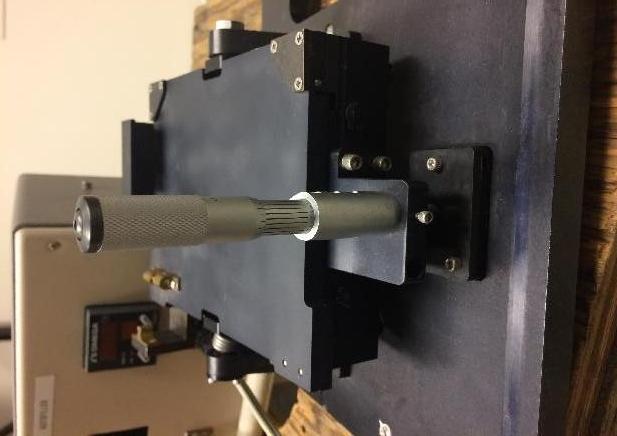
The grating tilt (and hence wavelength coverage) is adjusted with a manual, digital-readout micrometer. Each digit corresponds to a 0.001 inch adjustment. Two different styles of micrometers are used: the style used with the 300 and 600 gpm gratings has a locking ring, while the other style used for the 1200 gpm grating does not. We expect that the 1200 gpm grating micrometer has sufficient internal friction to prevent undesired rotation. Please alert us if you have any doubts on this score. Make sure to loosen the locking ring before you change the 300 or 600 micrometer settings! The locking ring is loosened with a counterclockwise rotation. Re-tighten the locking ring once you are at the desired setting. To find the micrometer setting for a given grating, use the grating calculator. The relations built into the calculator with λ in are:

300 gpm: Setting=0.0756 λ + 164

600 gpm: Setting=0.1679 λ - 356

1200 gpm with no spacer: Setting=0.3041 λ - 1585 -- measured & updated 12/22/09

1200 gpm with spacer (shown here, just below the tip of the micrometer): Setting=0.2853 λ - 1098 -- measured & updated 12/18/09

Please ask the staff to make sure the 11 mm (0.44 inch) spacer is in place if you wish to use the 1200 gpm grating in the blue. Note that there are 2 flat plates together that appear to be the spacer; the top plate is about 1.6 mm (0.06 inch) and must be left screwed in so the end of the micrometer will rest on it. Slightly improved thermal stability will be possible if you remove the 11 mm spacer for observations near H , but the convenience of not fussing with the spacer may override this modest gain.

If you wish to observe with the 1200 gpm grating, please note that to use a central wavelength beyond 7500A requires a special arrangement to tilt the grating to the desired angle. Please contact the staff, especially Wayne Peters, well in advance of your run.

6.0 Scattered Light
Scattered light in the spectrograph results from undesired reflections from the refractive optics and the CCD, imperfections in the reflective surfaces and scattering of light outside first order from the spectrograph case. We have minimized these sources of scattered light as far as we know how, but some remains. Scattered light amounting to 3% of the dispersed light is scattered fairly uniformly across the CCD surface. Only about 1% of this scattered light (or 0.03% of the dispersed light) will fall on top of the desired spectrum, but strong sky lines may contribute as well.

7.0 More on Resolution
Update by NC, 03/23/01 Note: this section uses measurements taken with the old FAST2.

The table in section 1.5 showing the resolution provided by various slit widths does not apply exactly to FAST2. In FAST2, electrons created in the silicon by blue light (and hence in the upper part of the silicon wafer) diffuse somewhat before reaching the buried channels.  The result is that comparison lines and other sharp features are broader in the blue than in the red. 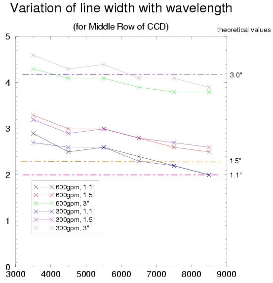Thus, the theoretical values reported in the section 1.5 table are not reached for the narrowest slits.   Below is a graph showing the measured resolutions for 3 different slits, as a function of wavelength.  Note that the most common slit used, the 3" slit, is affected by this property, but the achieved average is about equal to the theoretical value.  There is some variation of resolution as a function of position on the CCD, in the sense that the extreme ends of the spectrum are slightly poorer in resolution than the center (10%), and that the ends of the slit are also poorer (also about 10%).

The graph shows FWHM in pixels plotted against wavelength in angstroms.
 

Here is a table of measured resolutions, data of 2001.0322. Values quoted are FWHM in pixels .

                                      600gpm                                                    300gpm
                 1.1"                1.5"               3.0"                 1.1"            1.5"            3.0"
Wav
3500  2.9   2.9  2.9    3.3  3.3 3.6   4.3 4.3 4.5   2.9 2.7 3.0   3.2 3.2 3.5  4.5 4.6 5.1
4500  2.6   2.5  2.8    3.0  3.0 3.1   4.1 4.1 4.3   2.6 2.6 2.6   3.1 2.9 3.2  4.2 4.3 4.4
5500  2.5   2.6  3.0    3.0  3.0 3.1   4.3 4.1 4.4   2.5 2.6 2.9   3.1 3.0 3.3  4.3 4.4 4.6
6500  2.5   2.4  2.6    2.9  2.8 3.1   4.0 3.9 4.2   2.5 2.3 2.6   2.7 2.8 3.1  4.2 4.1 4.4
7500  2.3   2.2  2.4    2.7  2.6 2.9   3.9 3.8 4.0   2.3 2.2 2.5   2.7 2.7 2.9  4.0 4.1 4.2
8500  2.1   2.0  2.3    2.6  2.5 2.9   3.8 3.8 3.9   2.1 2.0 2.4   2.7 2.6 2.8  4.0 3.9 4.2

For each slit, the 3 columns represent values found for 3 different rows along the slit.  The row numbers in unbinned pixels are 60, 240, and 450.  

Similar, much more limited, measurements for FAST3 are shown in the table that follows. Widths are in asec, similar to pixels for binx2, 1 pix = 1.14". The trends for the widths are similar to those for FAST2. Rows for binx2 are 17, 70, 153.

# /fast/2014.0705/0067.COMP.fits - binx2 300gpm 
Wav     3" slit
A      widths (asec)
3870 4.87 4.82 4.83
5287 4.72 4.62 4.66
7278 4.52 4.39 4.40